Solution of Exam (F24), May 2024

by Jakob Lemvig and Steeven Hegelund Spangsdorf

from sympy import *
init_printing()
from dtumathtools import *

Exercise 1

Given quadratic form:

x1,x2,x3 = symbols("x_1 x_2 x_3")
xvec = Matrix([x1, x2, x3])
q = 5*x1**2 + 8*x1*x2 - 4*x1*x3 - 22*x1 + 5*x2**2 + 4*x2*x3 - 32*x2 + 8*x3**2 - 20*x3 + 53
q

a

The partial derivatives are:

qx1=diff(q,x1)
qx2=diff(q,x2)
qx3=diff(q,x3)

hence, the gradient is:

nabla_q = Matrix([qx1,qx2,qx3])
nabla_q

\[\begin{split}\displaystyle \left[\begin{matrix}10 x_{1} + 8 x_{2} - 4 x_{3} - 22\\8 x_{1} + 10 x_{2} + 4 x_{3} - 32\\- 4 x_{1} + 4 x_{2} + 16 x_{3} - 20\end{matrix}\right]\end{split}\]

for any \(\pmb{x}=(x_1,x_2,x_3) \in \mathbb{R}^3\). The gradient can also be found by:

nabla_q = dtutools.gradient(q,[x1,x2,x3])
nabla_q

\[\begin{split}\displaystyle \left[\begin{matrix}10 x_{1} + 8 x_{2} - 4 x_{3} - 22\\8 x_{1} + 10 x_{2} + 4 x_{3} - 32\\- 4 x_{1} + 4 x_{2} + 16 x_{3} - 20\end{matrix}\right]\end{split}\]

b

The Hessian matrix is computed by:

H_q = hessian(q, [x1,x2,x3])   # or dtutools.hessian(q, [x1,x2,x3])
H_q

\[\begin{split}\displaystyle \left[\begin{matrix}10 & 8 & -4\\8 & 10 & 4\\-4 & 4 & 16\end{matrix}\right]\end{split}\]

This completes the answer to question b. Using the Hessian matrix, it is easy to write the quadratic form in matrix form as:

A = S(1)/2 * H_q
b = Matrix([-22, -32, -20])
c = 53
A, b, c

\[\begin{split}\displaystyle \left( \left[\begin{matrix}5 & 4 & -2\\4 & 5 & 2\\-2 & 2 & 8\end{matrix}\right], \ \left[\begin{matrix}-22\\-32\\-20\end{matrix}\right], \ 53\right)\end{split}\]

q_check = xvec.T * A * xvec + b.T * xvec + Matrix([c])
q_check[0].simplify()

Indeed, the matrix form of \(q\) based on the Hessian matrix agrees with the given \(q\):

q_check[0].simplify() == q.simplify()

True

c

The Hessian is a real, symmetric matrix so we know according to the spectral theorem that there exists an orthonormal basis of eigenvectors. We find the eigenvalues and eigenvectors by:

eig = H_q.eigenvects()
eig

\[\begin{split}\displaystyle \left[ \left( 0, \ 1, \ \left[ \left[\begin{matrix}2\\-2\\1\end{matrix}\right]\right]\right), \ \left( 18, \ 2, \ \left[ \left[\begin{matrix}1\\1\\0\end{matrix}\right], \ \left[\begin{matrix}- \frac{1}{2}\\0\\1\end{matrix}\right]\right]\right)\right]\end{split}\]

The eigenvectors associated with different eigenvalues are orthogonal to each other since the matrix is real symmetric. However, since the algebraic multiplicity of the eigenvalue \(18\) is two, we need to make sure that the two associated linearly independent eigenvectors are orthogonal. We use the Gram-Schmidt procedure to obtain two orthonormal eigenvectors:

GramSchmidt(eig[1][2], True)

\[\begin{split}\displaystyle \left[ \left[\begin{matrix}\frac{\sqrt{2}}{2}\\\frac{\sqrt{2}}{2}\\0\end{matrix}\right], \ \left[\begin{matrix}- \frac{\sqrt{2}}{6}\\\frac{\sqrt{2}}{6}\\\frac{2 \sqrt{2}}{3}\end{matrix}\right]\right]\end{split}\]

The eigenvector associated with \(0\) only needs to be normalized. There are several ways to do this, e.g.,

GramSchmidt(eig[0][2], True)

\[\begin{split}\displaystyle \left[ \left[\begin{matrix}\frac{2}{3}\\- \frac{2}{3}\\\frac{1}{3}\end{matrix}\right]\right]\end{split}\]

or,

Matrix(eig[0][2]).normalized()

\[\begin{split}\displaystyle \left[\begin{matrix}\frac{2}{3}\\- \frac{2}{3}\\\frac{1}{3}\end{matrix}\right]\end{split}\]

Finally, we combine the three orthonormal eigenvectors in a basis denoted \(\beta\):

beta = GramSchmidt(eig[0][2], True)[0], GramSchmidt(eig[1][2], True)[0], GramSchmidt(eig[1][2], True)[1] 
beta

\[\begin{split}\displaystyle \left( \left[\begin{matrix}\frac{2}{3}\\- \frac{2}{3}\\\frac{1}{3}\end{matrix}\right], \ \left[\begin{matrix}\frac{\sqrt{2}}{2}\\\frac{\sqrt{2}}{2}\\0\end{matrix}\right], \ \left[\begin{matrix}- \frac{\sqrt{2}}{6}\\\frac{\sqrt{2}}{6}\\\frac{2 \sqrt{2}}{3}\end{matrix}\right]\right)\end{split}\]

The assoicated change-of-basis matrix \(Q\) is:

Q = Matrix([beta])
Q 

\[\begin{split}\displaystyle \left[\begin{matrix}\frac{2}{3} & \frac{\sqrt{2}}{2} & - \frac{\sqrt{2}}{6}\\- \frac{2}{3} & \frac{\sqrt{2}}{2} & \frac{\sqrt{2}}{6}\\\frac{1}{3} & 0 & \frac{2 \sqrt{2}}{3}\end{matrix}\right]\end{split}\]

Let’s check that \(Q\) is indeed an orthogonal matrix:

Q * Q.T

\[\begin{split}\displaystyle \left[\begin{matrix}1 & 0 & 0\\0 & 1 & 0\\0 & 0 & 1\end{matrix}\right]\end{split}\]

Note that \(Q\) is not unique (not even up to multiplication by \(-1\)) as there are infinitely many ways to obtain an orthonormal basis for the eigenspace associated with \(18\). Here is another change-of-basis matrix:

V = Matrix([[S(1)/3, S(-2)/3, S(2)/3], [S(2)/3, S(-1)/3, S(-2)/3], [S(2)/3, S(2)/3, S(1)/3]])
V * V.T, H_q * V, V

\[\begin{split}\displaystyle \left( \left[\begin{matrix}1 & 0 & 0\\0 & 1 & 0\\0 & 0 & 1\end{matrix}\right], \ \left[\begin{matrix}6 & -12 & 0\\12 & -6 & 0\\12 & 12 & 0\end{matrix}\right], \ \left[\begin{matrix}\frac{1}{3} & - \frac{2}{3} & \frac{2}{3}\\\frac{2}{3} & - \frac{1}{3} & - \frac{2}{3}\\\frac{2}{3} & \frac{2}{3} & \frac{1}{3}\end{matrix}\right]\right)\end{split}\]

d

We insert \(\pmb{x} = (1,2,1)\) in the expresseion of \(\nabla q\) which yields:

nabla_q.subs({x1:1,x2:2,x3:1})

\[\begin{split}\displaystyle \left[\begin{matrix}0\\0\\0\end{matrix}\right]\end{split}\]

Since the gradient at the given point is the zero vector, then \(\pmb{x} = (1,2,1)\) is a stationary point. To find all stationary points, we find all solutions to the equation system \(\nabla q(\pmb{x}) = (0,0,0)\):

solve(list(nabla_q),[x1,x2,x3])

Setting \(x_3 = t\), \(t \in \mathbb{R}\), we see that all stationary points are given by:

\[\begin{equation*} (x_1,x_2,x_3) = (2t-1, -2t+4, t) = (2,-2,1) t + (-1,4,0) \end{equation*}\]

where \(t \in \mathbb{R}\).

e

Since the function \(q\) is a quadratic form, the line found in question d above is a line along which there is no increase nor decrease of \(q\). In fact, this line is \((1,2,1) + \mathrm{span}(v_1)\) where \(v_1\) is an eigenvector of \(0\). So, the function \(q\) is constant in the direction of \(v_1\). Remark: The Hessian is not really useful here since:

H_q.eigenvals()

f

Given \(x_0\), and restating the gradient:

x0 = Matrix([1, 2, 1]) + 3 * V[:, 1]
nabla_q, x0

\[\begin{split}\displaystyle \left( \left[\begin{matrix}10 x_{1} + 8 x_{2} - 4 x_{3} - 22\\8 x_{1} + 10 x_{2} + 4 x_{3} - 32\\- 4 x_{1} + 4 x_{2} + 16 x_{3} - 20\end{matrix}\right], \ \left[\begin{matrix}-1\\1\\3\end{matrix}\right]\right)\end{split}\]

We carry out the gradient method to compute \(x_{10}\), where \(x_{n+1}=x_n-\alpha\nabla q(x_n)\) for \(n=0,1,2,\ldots\):

alpha = 0.02
x = x0
for n in range(1,11):
    x = x - alpha * nabla_q.subs({x1: x[0], x2: x[1], x3: x[2]})
x

\[\begin{split}\displaystyle \left[\begin{matrix}0.976941569907863\\1.98847078495393\\1.02305843009214\end{matrix}\right]\end{split}\]

The gradient method converges towards \((1,2,1)\) since 3 * V[:,1] belongs to the orthogonal complement of the null-space of \(A\). The gradient method progresses along this direction and intersects the “stationary line” at the point \((1,2,1)\).

Exercise 2

Given quadratic form:

x1, x2, x3, x4 = symbols("x_1 x_2 x_3 x_4")
q = 2 * x1 * x3 + 4 * x2 * x4
q

a

The Hessian matrix is given by:

H = hessian(q, [x1, x2, x3, x4])
H

\[\begin{split}\displaystyle \left[\begin{matrix}0 & 0 & 2 & 0\\0 & 0 & 0 & 4\\2 & 0 & 0 & 0\\0 & 4 & 0 & 0\end{matrix}\right]\end{split}\]

We note that the Hessian matrix is symmetric. A symmetric matrix \(A\) that fulfills \(q=\pmb{x}^TA\pmb{x}\), where \(\pmb{x}=[x_1,x_2,x_3,x_4]^T\) is thus:

A = S(1)/2 * H
A

\[\begin{split}\displaystyle \left[\begin{matrix}0 & 0 & 1 & 0\\0 & 0 & 0 & 2\\1 & 0 & 0 & 0\\0 & 2 & 0 & 0\end{matrix}\right]\end{split}\]

b

An orthogonal matrix \(Q\) that reduces the quadratic form is found as the change-of-basis matrix that diagonalizing \(A\):

Q, Lamda = A.diagonalize(normalize=True)
Q, Lamda

\[\begin{split}\displaystyle \left( \left[\begin{matrix}0 & - \frac{\sqrt{2}}{2} & \frac{\sqrt{2}}{2} & 0\\- \frac{\sqrt{2}}{2} & 0 & 0 & \frac{\sqrt{2}}{2}\\0 & \frac{\sqrt{2}}{2} & \frac{\sqrt{2}}{2} & 0\\\frac{\sqrt{2}}{2} & 0 & 0 & \frac{\sqrt{2}}{2}\end{matrix}\right], \ \left[\begin{matrix}-2 & 0 & 0 & 0\\0 & -1 & 0 & 0\\0 & 0 & 1 & 0\\0 & 0 & 0 & 2\end{matrix}\right]\right)\end{split}\]

Denote the \(i\)th column vector of \(Q\) by \(\pmb{q}_i\), and let \(\beta = \pmb{q}_1, \pmb{q}_2, \pmb{q}_3, \pmb{q}_4\).
Defining new coordinates as \(\pmb{k}=[k_1,k_2,k_3,k_4]^T\), where \(\pmb{k} = Q^T \pmb{x}\), we have \(q\) expressed in the reduced form:

k1, k2, k3, k4 = symbols("k_1,k_2,k_3,k_4")
kvec = Matrix([k1, k2, k3, k4])
q_new = Matrix([kvec.T * Lamda * kvec])[0]
q_new

c

We now consider \(q\) restricted to the set:

\[\begin{equation*} B=\{ \pmb{x}\in \mathbb{R}^4 \mid x_1^2+x_2^2+x_3^2+x_4^2\leq 1 \}. \end{equation*}\]

Since \(q: B \to \mathbb{R}\) is continuous on a bounded and closed domain, it has a global minimum and maximum value by Theorem 5.2.1.

d

Extrema of \(q\) over the domain \(B\) are to be found in the stationary points in the interior of \(B\), at the boundary of \(B\), or at exceptional points (see Theorem 5.2.2). Since the function is smooth, there are no exceptional points. Hence, we must investigate the interior and the boundary. First, the interior:

The partial derivatives are given by:

qx1 = diff(q, x1)
qx2 = diff(q, x2)
qx3 = diff(q, x3)
qx4 = diff(q, x4)
qx1, qx2, qx3, qx4

Thus, the gradient is:

nabla_q = Matrix([qx1, qx2, qx3, qx4])
nabla_q

\[\begin{split}\displaystyle \left[\begin{matrix}2 x_{3}\\4 x_{4}\\2 x_{1}\\4 x_{2}\end{matrix}\right]\end{split}\]

Alternatively, it can be found by:

nabla_q = dtutools.gradient(q, [x1, x2, x3, x4])
nabla_q

\[\begin{split}\displaystyle \left[\begin{matrix}2 x_{3}\\4 x_{4}\\2 x_{1}\\4 x_{2}\end{matrix}\right]\end{split}\]

Hence, obviuosly, the gradient equals the zero vector if and only if \(\pmb{x}=0\). We can check this in Python by:

solve(list(nabla_q), [x1, x2, x3, x4])

So, there exists only one stationary point in the interior of \(q\) on \(B\), and it is found at \((0,0,0,0)\). The corresponding function value is:

q.subs({x1: 0, x2: 0, x3: 0, x4: 0})

Now, investigating boundary points. We see from the given set that the boundary of \(B\) is a unit sphere centred at the origin with a radius of 1, so all points that fulfill \(x_1^2+x_2^2+x_3^2+x_4^2=1\):

\[\begin{equation*} \partial B=\{ \pmb{x}\in \mathbb{R}^4 \mid \Vert \pmb{x} \Vert = 1 \}. \end{equation*}\]

We note that this unit sphere \(\partial B\) is invariant under \(Q^T\) (and \(Q\)) since \(Q^T\) is orthogonal and therefore satisfies \(\Vert Q^T \pmb{x}\Vert = \Vert\pmb{x} \Vert\) for all \(\pmb{x}\) (see Theorem 2.6.1(vi)). Alternatively, you may argue using that \(Q^T\) only causes rotation and reflection of the coordinate system and does not alter distances. Hence, we may use the easier new coordinates, which we above denoted by \(\pmb{k}\), and the unit sphere is thus described by \(\Vert \pmb{k} \Vert = k_1^2+k_2^2+k_3^2+k_4^2=1\).

Recall that \(q\) in the new coordinates was:

q_new

Note that \(k_1,k_2,k_3,k_4\) are squared in this expression, so \(k_1,k_2\) have negative contributions, while \(k_3,k_4\) have positive contributions. Maximum of \(q\) on the sphere is thus found, firstly where \(k_1=0,k_2=0\), and secondly where \(k_4^2\) is largest due to its larger factor, meaning that \(k_4=\pm 1\) while \(k_3=0\). Maximum on the boundary is thus found at \(\pmb{k}=[0,0,0,1]^T\) and at \(\pmb{k}=[0,0,0,-1]^T\) with a function value of:

q_new.subs({k1: 0, k2: 0, k3: 0, k4: 1})

Equivalently, a minimum is found where \(k_3,k_4\) are zero and \(k_1^2\) is largest, so \(k_1=\pm 1\), thus requiring \(k_2=0\). Minimum on the boundary is thus found at \((1,0,0,0)\) and at \((-1,0,0,0)\) with a function value of:

q_new.subs({k1: 1, k2: 0, k3: 0, k4: 0})

The stationary point is seen to not be an extremum. Global extrema of \(q\) on \(B\) are hence on the boundary as found above. We are not asked to find the location of the extremas, but they are easily found in the standard basis using \(Q\)

Q * kvec.subs({k1: 0, k2: 0, k3: 0, k4: 1}), Q * kvec.subs({k1: 0, k2: 0, k3: 0, k4: -1})

\[\begin{split}\displaystyle \left( \left[\begin{matrix}0\\\frac{\sqrt{2}}{2}\\0\\\frac{\sqrt{2}}{2}\end{matrix}\right], \ \left[\begin{matrix}0\\- \frac{\sqrt{2}}{2}\\0\\- \frac{\sqrt{2}}{2}\end{matrix}\right]\right)\end{split}\]

Q * kvec.subs({k1: 1, k2: 0, k3: 0, k4: 0}), Q * kvec.subs({k1: -1, k2: 0, k3: 0, k4: 0})

\[\begin{split}\displaystyle \left( \left[\begin{matrix}0\\- \frac{\sqrt{2}}{2}\\0\\\frac{\sqrt{2}}{2}\end{matrix}\right], \ \left[\begin{matrix}0\\\frac{\sqrt{2}}{2}\\0\\- \frac{\sqrt{2}}{2}\end{matrix}\right]\right)\end{split}\]

which is the locations of the two maxima and the two minima, respectively.

Exercise 3

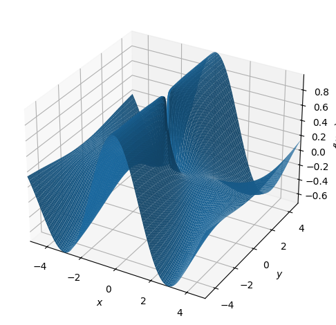
Given function \(f:\mathbb R^2\to\mathbb R\) which for \((x,y)=(0,0)\) is \(f(0,0)=0\), and for \((x,y)\in\mathbb R^2\setminus(0,0)\) is:

x,y = symbols("x y", real=True)
f = y**2 * cos(x) / (x**2 + y**2)
f

a

Plot for \((x,y)\in\mathbb R^2\setminus(0,0)\):

dtuplot.plot3d(f, (x, -5, 5), (y, -5, 5))

<spb.backends.matplotlib.matplotlib.MatplotlibBackend at 0x7f0578e8fa30>

b

First-order partial derivatives for \((x,y)\in\mathbb R^2\setminus(0,0)\) are found to be:

f.diff(x), f.diff(y)

c

2nd-degree Taylor polynomial \(P_2\) of \(\cos(x)\) expanded from \(x_0=0\):

series(cos(x), x, 0, 3).removeO()

d

Note first that \(f(x,x)\) is just a special case of \(f(x,y)\) where \(x=y\). The limit value is then easily computed:

\[\begin{equation*} \lim_{x\to 0}f(x,x)=\lim_{x\to 0}\frac{x^2\cos(x)}{x^2+x^2}=\lim_{x\to 0}\frac{\cos(x)}{2}= \frac12 \end{equation*}\]

Check:

f.subs(y,x).limit(x,0)

or (using Taylor’s limit formula):

(y**2 * series(cos(x), x, 0, 3).removeO() / (x**2 + y**2)).subs(y,x)

e

The limit value:

\[\begin{equation*} \lim_{x\to 0}f(x,2x)=\lim_{x\to 0}\frac{(2x)^2\cos(x)}{x^2+(2x)^2}=\lim_{x\to 0}\frac{4x^2\cos(x)}{x^2+4x^2}=\lim_{x\to 0}\frac{4\cos(x)}{5}=\frac45 \end{equation*}\]

Check:

f.subs(y,2*x).limit(x,0)

f

The first-order partial derivatives are continuously differentiable on \(\mathbb{R}^2 \setminus \{(0,0)\}\) so \(f\) is differentiable on this domain. Since \(f\) is not continuous at \((0,0)\), it is not differentiable here.

Exercise 4

Given vector field \(\pmb{V}\) and parametrization \(\pmb{r}(u)\) of a curve \(K_1\):

x, y, z, u, t = symbols("x y z u t", real=True)
V = Matrix([-x, x*y**2, x+z])
r = Matrix([u, u**2, u +1])
V, r

\[\begin{split}\displaystyle \left( \left[\begin{matrix}- x\\x y^{2}\\x + z\end{matrix}\right], \ \left[\begin{matrix}u\\u^{2}\\u + 1\end{matrix}\right]\right)\end{split}\]

where \(u\in[0,2]\).

a

Tangent vector \(\pmb{r}'(u)\):

rd = diff(r,u)
rd

\[\begin{split}\displaystyle \left[\begin{matrix}1\\2 u\\1\end{matrix}\right]\end{split}\]

This vector is never the zero vector (and \(\pmb{r}\) is obviously injective), hence the parametrization is regular.

b

The inner product of \(\pmb{V}(\pmb{r}(u))\) with \(\pmb{r}'(u)\) can be carried out as a usual dot product since all elements are real, \(\langle \pmb{V}(\pmb{r}(u)),\pmb{r}'(u) \rangle=\pmb{V}(\pmb{r}(u))\cdot \pmb{r}'(u)\). Hence, we get:

innerproduct = V.subs({x: r[0], y: r[1], z: r[2]}).dot(rd)
innerproduct.simplify()

The tangential line integral \(\int_{K_1}\pmb{V}\cdot \mathrm{d}\pmb{s}\) is given by:

integrate(innerproduct, (u, 0, 2))

c

As a parametrization \(K_2 = \pmb{p}([0,1])\) of the straight line segment \(K_2\) from \((0,0,1)\) to \((2,4,3)\) we use:

xstart = Matrix([0, 0, 1])
xend = Matrix([2, 4, 3])

p = xstart + t * (xend - xstart)
p

\[\begin{split}\displaystyle \left[\begin{matrix}2 t\\4 t\\2 t + 1\end{matrix}\right]\end{split}\]

where \(t\in[0,1]\).

The tangent vector \(\pmb{p}'(t)\):

pd = diff(p,t)
pd

\[\begin{split}\displaystyle \left[\begin{matrix}2\\4\\2\end{matrix}\right]\end{split}\]

The (tangential) line integral \(\int_{K_2}\pmb{V}\cdot \mathrm{d}\pmb{s}\), where the inner product again is a dot product, is:

innerproduct2 = V.subs({x: p[0], y: p[1], z: p[2]}).dot(pd)
innerproduct2.simplify()

integrate(innerproduct2, (t, 0, 1))

d

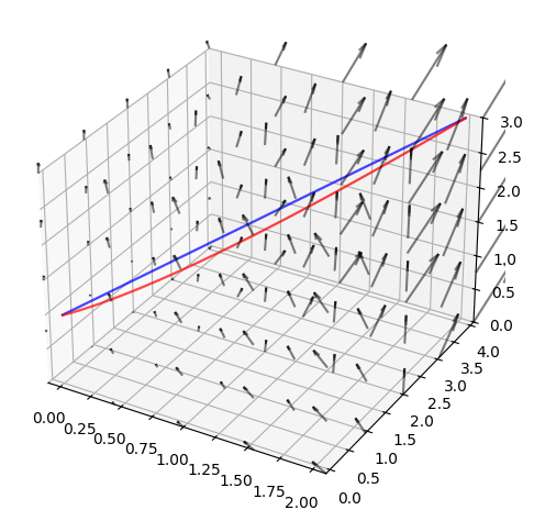
Looking back at the parametrization \(\pmb{r}(u) , u\in[0,2]\) of \(K_1\), we evaluate the \((x,y)\) coordinates of the end points:

r.subs({u:0}),r.subs({u:2})

\[\begin{split}\displaystyle \left( \left[\begin{matrix}0\\0\\1\end{matrix}\right], \ \left[\begin{matrix}2\\4\\3\end{matrix}\right]\right)\end{split}\]

We see that \(K_1\) and \(K_2\) are two curves with the same starting and end points. Thus, \(\pmb{V}\) is not a gradient vector field since the (tangential) line integral from \((0,0,1)\) to \((2,4,3)\) depends on the path, since we got different values in questions b and c (according to Lemma 7.4.1).

Alternatively, we can arrive at the same conclusion by showing that the Jacobian matrix is not symmetric (according to Lemma 7.3.2):

V.jacobian([x,y,z])

\[\begin{split}\displaystyle \left[\begin{matrix}-1 & 0 & 0\\y^{2} & 2 x y & 0\\1 & 0 & 1\end{matrix}\right]\end{split}\]

Some illustrative plots (not asked for)

K1 = dtuplot.plot3d_parametric_line(
    *r, (u,0,2), show=False, rendering_kw={"color": "red"}, colorbar=False
)
K2 = dtuplot.plot3d_parametric_line(
    *p, (t,0,1), show=False, rendering_kw={"color": "blue"}, colorbar=False
)
vektorfelt_V = dtuplot.plot_vector(
    V,
    (x, -.1, 2.1),
    (y, -.1, 4.1),
    (z, 0, 3),
    n=5,
    quiver_kw={"alpha": 0.5, "length": 0.05, "color": "black"},
    colorbar=False,
    show=False,
)

combined = K1 + K2 + vektorfelt_V
combined.legend = False
combined.show()

Exercise 5

Consider the function \(f: \mathbb{R}^2 \to \mathbb{R}\) given by

\[\begin{equation*} f(x_1,x_2) = x_1^2 +x_2^2 + x_1 +1 \end{equation*}\]

and the subset \(A \subset \mathbb{R}^2\) given by:

\[\begin{equation*} A = \{(x_1 ,x_2 )\in \mathbb{R}^2 \mid -2\leq x_1 \leq 2 \, \wedge \, -1\leq x_2 \leq 1 \}. \end{equation*}\]

a

We compute the integral \(\int_{A} f(x_1,x_2) \,\mathrm{d} (x_1,x_2)\) by:

x1, x2 = symbols("x_1 x_2", real=True)
f = x1**2 + x2**2 + x1 + 1
integrate(f, (x1,-2,2), (x2,-1,1))

b

Determining the volume of the set

\[\begin{equation*} \{(x_1,x_2,x_3)\in \mathbb{R}^3 \mid (x_1,x_2) \in A \wedge 0\leq x_3 \leq f(x_1 ,x_2) \}. \end{equation*}\]

We first plot the graph of \(f\):

dtuplot.plot3d(f, (x1, -2, 2), (x2, -1, 1))

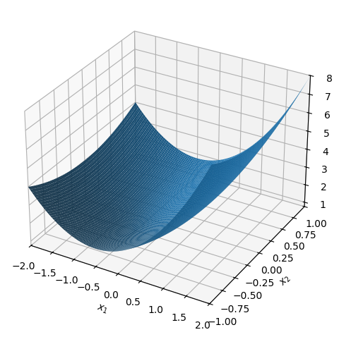
<spb.backends.matplotlib.matplotlib.MatplotlibBackend at 0x7f0558254670>

and note that \(f\) is positive on \(A\). Since \(f\) is positive on \(A\), then \(f\) resembles an elevation function. The volume is thus equal to the integral found in question a, i.e. \(64/3\).

c

Let \(a > 0\). Let \(B \subset \mathbb{R}^2\) denote the circular disk with center at the origin and radius \(a\):

\[\begin{equation*} B=\{(x_1 ,x_2 )\in \mathbb{R}^2 \mid x_1^2 + x_2^2 \le a^2\}. \end{equation*}\]

Parametrizing \(B\) using polar coordinates \((r,\theta)\) as:

\[\begin{equation*} s(r,\theta)=(r\cos(\theta),r\sin(\theta)) \end{equation*}\]

where \(r \in [0,a] , \theta \in [0, 2\pi[\). Hence, we can write \(B\) as:

\[\begin{equation*} B=\{(r \cos(\theta) ,r \sin(\theta) )\in \mathbb{R}^2 \mid r \in [0,a] \wedge \theta \in [0, 2\pi[ \}. \end{equation*}\]

r, theta = symbols("r theta", real=True)
s = Matrix([r * cos(theta), r * sin(theta)])
s

\[\begin{split}\displaystyle \left[\begin{matrix}r \cos{\left(\theta \right)}\\r \sin{\left(\theta \right)}\end{matrix}\right]\end{split}\]

The partial derivatives of \(s\) is given by:

sr = s.diff(r)
stheta = s.diff(theta)
sr, stheta

\[\begin{split}\displaystyle \left( \left[\begin{matrix}\cos{\left(\theta \right)}\\\sin{\left(\theta \right)}\end{matrix}\right], \ \left[\begin{matrix}- r \sin{\left(\theta \right)}\\r \cos{\left(\theta \right)}\end{matrix}\right]\right)\end{split}\]

and the Jacobian determinant is therefore:

Jac_det = Matrix.hstack(sr, stheta).det().simplify()
Jac_det

d

To determine the value of \(a\) to 3 decimal places such that

\[\begin{equation*} \int_{A} f(x_1,x_2) \,\mathrm{d} (x_1,x_2)=\int_{B} f(x_1,x_2) \,\mathrm{d} (x_1,x_2) \end{equation*}\]

we must compute the right-hand side’s plane integral \(\int_{B} f(x_1,x_2) \,\mathrm{d} (x_1,x_2)\).

Since the Jacobian determinant is non-zero in the interior of \(B\), and since the parametrization is regular (injective and never the zero vector on the interior of \(B\)), we can carry out the integral over the parameter region with the Jacobian function as a correction factor.

The Jacobian function is the absolute value of the Jacobian determinant. The determinant is \(r\) and thus always non-negative, so the Jacobian function is just:

Jac = r

The integrand of the plane integral of \(f\) over \(B\):

a = symbols("a", real=True)
integrand = Jac_det * f.subs({x1: r * cos(theta), x2: r * sin(theta)}).simplify()
integrand

The plane integral \(\int_{B} f(x_1,x_2) \,\mathrm{d} (x_1,x_2)\):

int_value = integrate(integrand, (theta, 0, 2* pi), (r,0,a))
int_value

Hence, \(\int_{A} f(x_1,x_2) \,\mathrm{d} (x_1,x_2)=\int_{B} f(x_1,x_2) \,\mathrm{d} (x_1,x_2)\) happens exactly when \(64/3=\frac{\pi a^4}2+\pi a^2\). Thus, we can find the value of \(a>0\) that results in \(\int_{A} f(x_1,x_2) \,\mathrm{d} (x_1,x_2)=\int_{B} f(x_1,x_2) \,\mathrm{d} (x_1,x_2)\) by:

sols = solve(Eq(int_value, S(64) / 3))
sols

sols[0].evalf(),sols[1].evalf()

Hence, since \(a>0\), we conclude that \(a = 1.679\).