Solution to re-exam (F24), August 2024

By shsp and jakle @ DTU Compute

from sympy import *

init_printing()
from dtumathtools import *

Exercise 1

Consider the function \(f: \mathbb{R}^2 \to \mathbb{R}\) given by

\[\begin{equation*} f(x,y) = 2 x^2 + y^2 - x y^2. \end{equation*}\]

x, y = symbols("x y", real=True)
f = 2 * x**2 + y**2 - x * y**2

f

(a)

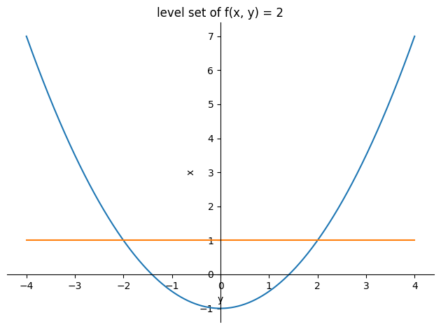
The level set \(\{(x,y)\in\mathbb R^2|f(x,y)=2\}\) is constituted by:

solve(Eq(f, 2)), solveset(Eq(f, 2), x)

This level set consists of the vertical line \(x=1\) and the parabola \(x=\frac12 y^2-1.\) Plotted in a \((y,x)\) coordinate system (note that the axes have been switched):

plot(
    y**2 / 2 - 1,
    1,
    (y, -4, 4),
    xlabel="y",
    ylabel="x",
    title="level set of f(x, y) = 2",
)

<sympy.plotting.backends.matplotlibbackend.matplotlib.MatplotlibBackend at 0x7f55b5f95dc0>

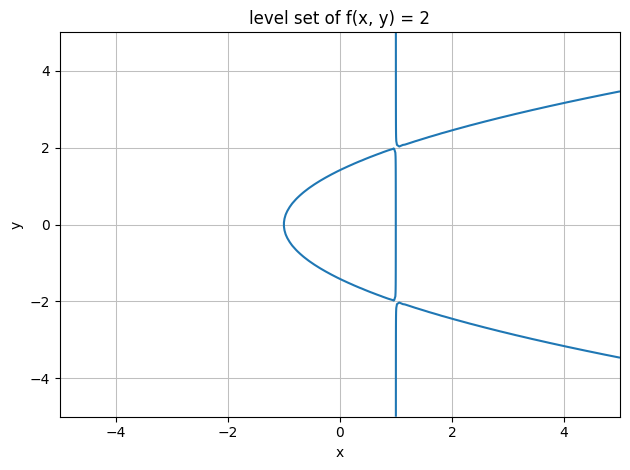
To plot it in the more usual \((x,y)\) coordinate system, we have to use plot_implicit:

dtuplot.plot_implicit(
    Eq(f, 2),
    (x, -5, 5),
    (y, -5, 5),
    xlabel="x",
    ylabel="y",
    title="level set of f(x, y) = 2",
)

<spb.backends.matplotlib.matplotlib.MatplotlibBackend at 0x7f5595034a30>

(b)

We can compute the gradient \(\nabla f(x,y)\) for all \((x,y) \in \mathbb{R}^2\) directly by:

grad = dtutools.gradient(f)
grad

\[\begin{split}\displaystyle \left[\begin{matrix}4 x - y^{2}\\- 2 x y + 2 y\end{matrix}\right]\end{split}\]

(c)

We can compute the Hessian matrix \(\pmb{H}_f(x,y)\) for all \((x,y) \in \mathbb{R}^2\) directly by:

H = dtutools.hessian(f)
H

\[\begin{split}\displaystyle \left[\begin{matrix}4 & - 2 y\\- 2 y & 2 - 2 x\end{matrix}\right]\end{split}\]

(d)

At a stationary point, the gradient equals \((0,0).\) Testing for the point \((0,0)\):

grad.subs({x:0,y:0})

\[\begin{split}\displaystyle \left[\begin{matrix}0\\0\end{matrix}\right]\end{split}\]

We see that \((0,0)\) indeed is a stationary point.

Hessian matrix eigenvalues:

Hlambdas = Matrix(list(H.eigenvals()))
Hlambdas

\[\begin{split}\displaystyle \left[\begin{matrix}- x - \sqrt{x^{2} + 2 x + 4 y^{2} + 1} + 3\\- x + \sqrt{x^{2} + 2 x + 4 y^{2} + 1} + 3\end{matrix}\right]\end{split}\]

Eigenvalues of the Hessian matrix at \((0,0)\):

Hlambdas.subs({x: 0, y: 0})

\[\begin{split}\displaystyle \left[\begin{matrix}2\\4\end{matrix}\right]\end{split}\]

According to Theorem 5.2.4, with two positive eigenvalues of the corresponding Hessian matrix, the stationary point \((0,0)\) is a local minimum.

(e)

All stationary points by solving for when both partial derivatives are zero simultaneously:

solve([Eq(grad[0], 0), Eq(grad[1], 0)])

So, \(f\) has the three stationary points \((0,0)\), \((1,-2)\), \((1,2).\)

Hessian matrix eigenvalues at the two latter stationary points:

Hlambdas.subs({x: 1, y: -2}).evalf()

\[\begin{split}\displaystyle \left[\begin{matrix}-2.47213595499958\\6.47213595499958\end{matrix}\right]\end{split}\]

Hlambdas.subs({x: 1, y: -2}).evalf()

\[\begin{split}\displaystyle \left[\begin{matrix}-2.47213595499958\\6.47213595499958\end{matrix}\right]\end{split}\]

Both of these stationary points \((1,-2),(1,2)\) show eigenvalues of opposite signs of their corresponding Hessian matrices. According to the Theorem, they are both saddle points. With \((0,0)\) found to be a local minimum above, all stationary points have now been covered for.

Exercise 2

Given column vector \(\boldsymbol y\) in \(\mathbb R^4\) equipped with the standard inner product:

y = Matrix([1, 2, 2, 4])
y

\[\begin{split}\displaystyle \left[\begin{matrix}1\\2\\2\\4\end{matrix}\right]\end{split}\]

(a)

Creating the matrix \(A=\boldsymbol y \boldsymbol y^T\):

A = y * y.T
A

\[\begin{split}\displaystyle \left[\begin{matrix}1 & 2 & 2 & 4\\2 & 4 & 4 & 8\\2 & 4 & 4 & 8\\4 & 8 & 8 & 16\end{matrix}\right]\end{split}\]

The transpose matrix \(A^T\):

A.transpose()

\[\begin{split}\displaystyle \left[\begin{matrix}1 & 2 & 2 & 4\\2 & 4 & 4 & 8\\2 & 4 & 4 & 8\\4 & 8 & 8 & 16\end{matrix}\right]\end{split}\]

According to the list on page 6 in the textbook, since \(A=A^T\) then the matrix \(A\) is symmetric.

An alternative general argument is as follows: Any matrix of the form \(Y Y^T\) is symmetric where \(Y\) is a matrix (or vector). The proof is easy:

\[\begin{equation*} (Y Y^T)^T = (Y^T)^T Y^T = Y Y^T \end{equation*}\]

(b)

We see easily that the second and third columns are formed by multiplying the first column by the scalar \(2\), and likewise the fourth column by the scalar \(4\). Hence all columns are scalar multiples of each other. Again, it is possible to give a more general argument. Let \(A\) be any matrix of the form \(\pmb{y} \pmb{y}^T\). Then

\[\begin{equation*} A = \pmb{y} \pmb{y}^T = \pmb{y} [y_1 y_2 \cdots y_n]^T = [\pmb{y} y_1 \, \pmb{y} y_2 \, \cdots \, \pmb{y} y_n] \end{equation*}\]

which shows that all columns are scalar mulitples of \(\pmb{y}\).

It follows that any linear combination of columns of \(A\) will belong to \(\mathrm{span}(\pmb{y})\). Therefore, the rank of the matrix will be \(\rho(A)=1\) since the rank is the dimension of span of the columns (i.e., the number of columns that are linearly independent as vectors). We check this:

A.rank()

(c)

For \(\mathbb R^4\), the inner product is given by: \(\langle \boldsymbol x,\boldsymbol y \rangle=\boldsymbol x\cdot \boldsymbol y = \boldsymbol y ^T \pmb{x}\).

Hence, we look for a non-zero vector \(\boldsymbol x\in \mathbb R^4\) such that \(\boldsymbol y ^T \pmb{x} = 0\). A vector that fulfills this could be:

x = Matrix([2, -1, 0, 0])
x

\[\begin{split}\displaystyle \left[\begin{matrix}2\\-1\\0\\0\end{matrix}\right]\end{split}\]

We check:

x.dot(y)

or, alternatively:

y.T * x

\[\displaystyle \left[\begin{matrix}0\end{matrix}\right]\]

(d)

We have:

\[\begin{equation*} 0 = \langle\boldsymbol x,\boldsymbol y \rangle = \boldsymbol y^T \boldsymbol x, \end{equation*}\]

where the last expression is a vector multiplication. Therefore

\[\begin{equation*} A \pmb{x} = \boldsymbol y \boldsymbol y^T \boldsymbol x = \boldsymbol y 0 = \pmb{0} \end{equation*}\]

(e)

The subspace spanned by \(\boldsymbol y\) is denoted \(Y=\mathrm{span}(\boldsymbol y)\). Its orthogonal complement is given to be \(Y^\perp=\mathrm{ker}A\).

According to the rank-nullity theorem (in Danish: the dimension theorem):

\[\begin{equation*} \mathrm{dim}(\mathbb R^4)=\mathrm{dim}(\mathrm{ker}A)+\rho(A). \end{equation*}\]

We therefore have that \(4=\mathrm{dim}(Y^\perp)+1\). Hence, \(\mathrm{dim}(Y^\perp)=3\).

(f)

A basis for \(Y^\perp\) is a basis for \(\mathrm{ker} A\) and will contain \(3\) basis vectors due to its dimension. We find such a basis for \(\mathrm{ker}A\) by solving \(A\boldsymbol x=\boldsymbol 0,\) quickly done with Sympy:

sols = A.nullspace()
sols

\[\begin{split}\displaystyle \left[ \left[\begin{matrix}-2\\1\\0\\0\end{matrix}\right], \ \left[\begin{matrix}-2\\0\\1\\0\end{matrix}\right], \ \left[\begin{matrix}-4\\0\\0\\1\end{matrix}\right]\right]\end{split}\]

We perform the GramSchmidt procedure to generate an orthonormal basis vector set spanning the same subspace:

sols_ortho = GramSchmidt(sols, True)
sols_ortho

\[\begin{split}\displaystyle \left[ \left[\begin{matrix}- \frac{2 \sqrt{5}}{5}\\\frac{\sqrt{5}}{5}\\0\\0\end{matrix}\right], \ \left[\begin{matrix}- \frac{2 \sqrt{5}}{15}\\- \frac{4 \sqrt{5}}{15}\\\frac{\sqrt{5}}{3}\\0\end{matrix}\right], \ \left[\begin{matrix}- \frac{4}{15}\\- \frac{8}{15}\\- \frac{8}{15}\\\frac{3}{5}\end{matrix}\right]\right]\end{split}\]

v1 = sols_ortho[0]
v2 = sols_ortho[1]
v3 = sols_ortho[2]
v1, v2, v3

\[\begin{split}\displaystyle \left( \left[\begin{matrix}- \frac{2 \sqrt{5}}{5}\\\frac{\sqrt{5}}{5}\\0\\0\end{matrix}\right], \ \left[\begin{matrix}- \frac{2 \sqrt{5}}{15}\\- \frac{4 \sqrt{5}}{15}\\\frac{\sqrt{5}}{3}\\0\end{matrix}\right], \ \left[\begin{matrix}- \frac{4}{15}\\- \frac{8}{15}\\- \frac{8}{15}\\\frac{3}{5}\end{matrix}\right]\right)\end{split}\]

Checking for orthogonality (inner products, meaning dot products, must be 0) and magnitudes of 1:

v1.dot(v2), v2.dot(v3), v3.dot(v1)

v1.norm(), v2.norm(), v3.norm()

Fulfilled, hence they constitute an orthonormal basis for \(Y^\perp\).

Exercise 3

Let the function \(f : \mathbb{R} \to \mathbb{R}\) be given by

\[\begin{equation*} f(x) = \begin{cases} \frac{\sin(x)}{x} & \text{for } x \neq 0, \\ 1 & \text{for } x = 0. \end{cases} \end{equation*}\]

x = symbols("x", real=True)
f = sin(x) / x

(a)

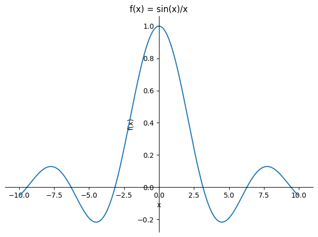
Plot of the graph for \(x \in [-10,10]\):

plot(f, (x, -10, 10), ylabel="f(x)", xlabel="x", title="f(x) = sin(x)/x")

<sympy.plotting.backends.matplotlibbackend.matplotlib.MatplotlibBackend at 0x7f5594d87fd0>

The plot shows the graph of \(f(x)\) for \(x\neq 0\). For \(x=0\), the point \((0,1)\) should be added to the plot for completeness.

We consider \(x=k\pi\) for each \(k\in\mathbb Z\):

• For \(k=0\), we have \(x=0\), and thus we are in the second case where \(f(0)=1.\)

• For each \(k\in\mathbb Z\setminus\{0\}\) we are in the first case. Since \(\sin(k\pi)=0\) for any integer \(k\), then \(f(k\pi)=\frac{\sin(k\pi)}{kx}=0\) for each \(k\in\mathbb Z\setminus\{0\}\).

We conclude that:

\[\begin{equation*} f(k \pi) = \begin{cases} 0 & \text{for } k \neq 0, \\ 1 & \text{for } k = 0. \end{cases} \end{equation*}\]

(b)

Second-degree Taylor polynomial of \(\sin(x)\) from expansion point \(x_0=0\):

sin(x).series(x, 0, 3).removeO()

So, the second-degree Taylor polynomial is \(P_2(x)=x.\)

(c)

For Taylor’s limit formula of \(\sin(x)\) from expansion point \(x_0=0\) we add the remainder term to the approximating polynomial from (b) according to Theorem 4.6.1:

\[\begin{equation*} \sin(x)=x+(x-x_0)^2\varepsilon(x-x_0)=x+x^2\varepsilon(x). \end{equation*}\]

The limit is:

\[\begin{equation*} \lim_{x\to0}\frac{\sin(x)}{x}=\lim_{x\to0}\frac{x+x^2\varepsilon(x)}{x}=\lim_{x\to0}(1+x\varepsilon(x))=1, \end{equation*}\]

since \(\varepsilon(x)\to0\) for \(x\to0\) by definition.

(d)

We know that \(\sin(x)\) and \(1/x\) are smooth functions for all \(x\neq0\), and thus continuous functions on that interval. According to the first bullet point on page 66 in the textbook, their product \(\sin(x)/x\) is thus also continuous for all \(x\neq0\). For \(x\to0\) we know from (c) that \(\sin(x)/x\to1\), but by definition we also have \(f(0)=1\). We therefore have continuity at \(x=0\). Hence, \(f\) is continuous at all \(x\in\mathbb R\), so \(f\) is a continuous function according to Definition 3.1.1.

(e)

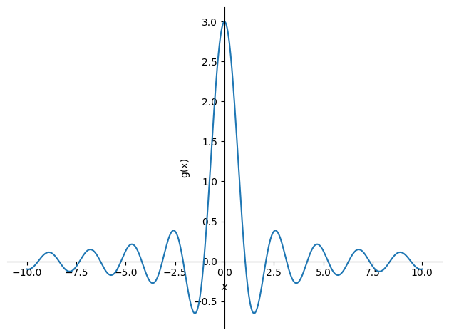
Given a function \(g:\mathbb R\to\mathbb R\) where \(g(x)=\sin(3x)/x\) for \(x\neq0\) and \(g(x)=c\) for \(x=0.\)

g = sin(3 * x) / x

Taylor’s limit formula of \(\sin(3x)\), choosing expansion point \(x_0=0\):

sin(3 * x).series(x, 0, 3)

So, Taylor’s limit formula is \(\sin(3x)=3x+x^2\varepsilon(x).\) Finding the limit:

\[\begin{equation*} \lim_{x\to0}\frac{\sin(3x)}{x}=\lim_{x\to0}\frac{3x+x^2\varepsilon(x)}{x}=\lim_{x\to0}(3+x\varepsilon(x))=3. \end{equation*}\]

Hence, if \(c=3\) then \(g\) is a continuous function.

Plot:

plot(g, (x, -10, 10), ylabel="g(x)")

<sympy.plotting.backends.matplotlibbackend.matplotlib.MatplotlibBackend at 0x7f5594d25e80>

Exercise 4

Consider the subset \(A \subset \mathbb{R}^2\) given by:

\[\begin{equation*} A = \{(x_1 ,x_2 )\in \mathbb{R}^2 \mid 1 \le x_1^2 +x_2^2 \le 4 \wedge x_1 \ge 0 \wedge x_2 \ge 0\}. \end{equation*}\]

Define the function \(f: A \to \mathbb{R}\) by

\[\begin{equation*} f(x_1,x_2) = \ln(x_1^2 +x_2^2). \end{equation*}\]

x1, x2 = symbols("x1 x2", real=True)
f = ln(x1**2 + x2**2)

(a)

To show that \(r^2 \ln(r^2) -r^2\) is an anti-derivative of \(2 \ln(r^2) r\), we simply have to verify that \(\left(r^2\ln(r^2)-r^2\right)' = 2r\ln(r^2)\). This is easily done:

r = symbols("r", real=True, positive=True)
exp = r**2 * ln(r**2) - r**2
exp.diff(r)

Of course, it is also possible to differentiate \(r^2\ln(r^2)-r^2\) by hand:

\[\begin{equation*} \left(r^2\ln(r^2)-r^2\right)'=\left(r^2\ln(r^2)\right)'-2r=(r^2)'\ln(r^2)+r^2\left(\ln(r^2)\right)'-2r=2r\ln(r^2)+r^2\left(\ln(r^2)\right)'-2r. \end{equation*}\]

Here the product rule was used. We compute \(\left(\ln(r^2)\right)'\) using the chain rule, where we temporarily substitute in \(u=r^2\) as the inner function in the logarithm:

\[\begin{equation*} \left(\ln(r^2)\right)'=(r^2)'\left(\ln(u)\right)'=2r\frac1u=2r\frac1{r^2}=2/r. \end{equation*}\]

Continuing from where we left off before:

\[\begin{equation*} \left(r^2\ln(r^2)-r^2\right)'=2r\ln(r^2)+r^22/r-2r=2r\ln(r^2)+r2-2r=2r\ln(r^2). \end{equation*}\]

As we wanted to show.

(b)

Since we know from (a) that \(r^2\ln(r^2)-r^2\) is an antiderivative of \(2r\ln(r^2)\) for \(r>0\), then all antiderivatives when \(r>0\) are given by:

\[\begin{equation*} \int 2r\ln(r^2)\mathrm dr=r^2\ln(r^2)-r^2+k, \end{equation*}\]

where \(k\in\mathbb R\) is an arbitrary constant.

(c)

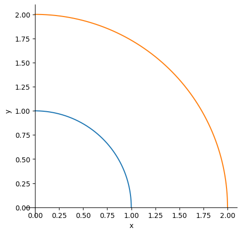
The set \(A\) is the quarter of an annulus (a “circle ring”) with inner radius 1 to outer radius 2 that is located in the first quadrant. Parametrization:

\[\begin{equation*} \boldsymbol p(r,\theta)=(r\cos(\theta),r\sin(\theta))\quad,\quad r\in[1,2],\theta\in[0,\pi/2]. \end{equation*}\]

theta = symbols("theta", real=True)
p = Matrix([r * cos(theta), r * sin(theta)])
p

\[\begin{split}\displaystyle \left[\begin{matrix}r \cos{\left(\theta \right)}\\r \sin{\left(\theta \right)}\end{matrix}\right]\end{split}\]

Plotting the inner and outer circle sections - the region \(A\) is the set of points between the two shown curves, bounded by the axes in the first quadrant:

p1 = plot_parametric(*p.subs({r:1}), (theta, 0, pi/2), xlabel="x", ylabel="y", aspect_ratio = (1,1), show=False)
p2 = plot_parametric(*p.subs({r:2}), (theta, 0, pi/2), show=False)
p1.extend(p2)
p1.show()

Partial derivatives of the parametrization:

p_r = p.diff(r)
p_theta = p.diff(theta)
p_r, p_theta

\[\begin{split}\displaystyle \left( \left[\begin{matrix}\cos{\left(\theta \right)}\\\sin{\left(\theta \right)}\end{matrix}\right], \ \left[\begin{matrix}- r \sin{\left(\theta \right)}\\r \cos{\left(\theta \right)}\end{matrix}\right]\right)\end{split}\]

Hence, the Jacobian matrix is:

J = p.jacobian([r,theta])
J

\[\begin{split}\displaystyle \left[\begin{matrix}\cos{\left(\theta \right)} & - r \sin{\left(\theta \right)}\\\sin{\left(\theta \right)} & r \cos{\left(\theta \right)}\end{matrix}\right]\end{split}\]

and the Jacobian determinant is:

detJ = J.det().simplify()
detJ

(d)

\(f\) is a continuous function for \(x_1^2+x_2^2>0\), so within the given region \(A\). A continuous function satisfying the conditions (I) and (II) on page 140 in the textbook is Riemann integrable according to the remark after Definition 6.3.1.

• \(A\) is bounded, so condition (I) is fulfilled.

• The boundary \(\partial A\) is formed by a continuously differentiable curve, since it is a circle with a parametrization \(\boldsymbol r\) as found in (c). Thus, condition (II) is fulfilled.

We conclude that \(f\) is Riemann integrable.

(e)

\(\boldsymbol p\) found in (c) is injective and has non-zero Jacobian determinant on \(\Gamma\). To compute the integral \(\int_Af(x_1,x_2)\mathrm d(x_1,x_2)\), we can therefore use the change-of-variables theorem 6.4.1:

\[\begin{equation*} \int_Af(x_1,x_2)\mathrm d(x_1,x_2)=\int_\Gamma f(\boldsymbol p(r,\theta))\,|\mathrm{det}(J_{\boldsymbol p}(r,\theta))|\,\mathrm d(r,\theta)=\int_1^2\int_0^{\pi/2} f(\boldsymbol p(r,\theta))\,|\mathrm{det}(J_{\boldsymbol p}(r,\theta))|\,\mathrm d\theta \mathrm dr, \end{equation*}\]

where \(J_{\boldsymbol p}\) is the Jacobian matrix.

Restriction \(f(\boldsymbol r(u,v)):\)

fr = f.subs({x1: p[0], x2: p[1]}).simplify()
fr

Plane integral:

integrate(fr * detJ, (theta, 0, pi / 2), (r, 1, 2)).expand()

Since

fr * detJ

we can also use the results in (a) to compute the plane integral as:

int_via_anti = S(1)/2 * (pi / 2 - 0) * (exp.subs({r: 2}) - exp.subs({r: 1}))
int_via_anti.expand()

The approximate value is:

_.evalf()